Source Reading 008 · GPU Profiling Internals源码阅读 008 · GPU Profiling 内核
Reading the Trace读懂这条 Trace
A field guide to AMD's instruction-level profiler: how rocprofv3 captures Advanced Thread Trace, and how to read every panel of rocprof-compute-viewer.一份 AMD 指令级 profiler 的实战指南:rocprofv3 如何采集 Advanced Thread Trace,以及 rocprof-compute-viewer 的每一块面板到底怎么看。
00Prologue序章
A counter tells you a kernel is slow. A trace tells you which instruction is waiting, and for what.计数器告诉你 kernel 慢了。 Trace 告诉你是哪条指令在等,以及在等什么。
Most GPU profiling stops at aggregates: occupancy, achieved bandwidth, a flat list of the top kernels. Useful, but it answers how much, never where. To optimize a hand-written kernel you need the other axis — the instruction stream of a single wave on a single SIMD, with a cycle cost stamped on every line. On AMD that axis is Advanced Thread Trace (ATT), a hardware feature of the SQ (sequencer) that records what each wave issued and how long it stalled.大多数 GPU profiling 止步于聚合量:occupancy、 实测带宽、 一张 top kernel 排行榜。 有用,但它只回答 多少,从不回答 在哪。 要优化一个手写 kernel,你需要另一条轴 —— 单个 SIMD 上单个 wave 的指令流,每一行都盖着 cycle 开销的时间戳。 在 AMD 上,这条轴就是 Advanced Thread Trace(ATT):SQ(sequencer)的一项硬件能力,记录每个 wave 发射了什么、 stall 了多久。
Two tools own that axis. rocprofv3 — the CLI inside rocprofiler-sdk — arms the hardware, runs your app, and decodes the raw token stream. rocprof-compute-viewer (RCV) — a Qt desktop app — turns the decode into a navigable picture: waterfall timelines per SIMD, an annotated ISA listing, a hotspot histogram, hardware-counter overlays. This reading is a guided tour of both, grounded in their source and in real traces captured on this box's MI350X.两个工具掌管这条轴。rocprofv3 —— rocprofiler-sdk 里的 CLI —— 负责武装硬件、 跑你的程序、 再解码原始 token 流。rocprof-compute-viewer(RCV)—— 一个 Qt 桌面程序 —— 把解码结果变成可导航的图景:每个 SIMD 的瀑布时间线、 带注释的 ISA 列表、 hotspot 直方图、 硬件计数器叠加。 这篇阅读就是带你走一遍这两个工具,落在它们的源码和这台机器 MI350X 上真实抓到的 trace 上。
01The pipeline数据管线
Five stages turn a running kernel into a panel you can click.五个阶段,把一个正在运行的 kernel 变成你能点击的面板。
The two tools are not one program — they are the front and back of a pipeline that hands a directory of JSON between them. Understanding the stages tells you exactly which knob lives where: capture parameters belong to rocprofv3, decode quality to the trace-decoder, everything visual to RCV.这两个工具不是一个程序 —— 它们是一条管线的前后两端,中间靠一个 JSON 目录交接。 看清这几个阶段,你就知道每个旋钮归谁管:采集参数属于 rocprofv3,解码质量属于 trace-decoder,所有可视化都归 RCV。
App → rocprofv3 --att (capture) → ROCprof Trace Decoder (runs automatically) → a ui_output_agent_* directory of per-wave JSON → opened by RCV. A stats_*.csv falls out on the side.应用 → rocprofv3 --att(采集)→ ROCprof Trace Decoder(自动运行)→ 一个 ui_output_agent_* 的 per-wave JSON 目录 → 由 RCV 打开。 旁路还会落一份 stats_*.csv。
rocprofv3 command and the RCV window. The middle only resurfaces when you build RCV from source and choose a decoder backend.解码这一步在采集后会 自动 运行,所以日常你只碰两端 —— rocprofv3 命令和 RCV 窗口。 中间那段只有在你从源码构建 RCV、 选择 decoder 后端时才会重新冒出来。02rocprofv3 — the front endrocprofv3 —— 前端
One CLI, four jobs: trace APIs, dispatch timing, hardware counters, and the thread trace.一个 CLI,四件活:trace API、 dispatch 计时、 硬件计数器,以及 thread trace。
rocprofv3 is the command-line front of rocprofiler-sdk — the rewrite of the old rocprof. It profiles an unmodified binary: you prefix your run with it and pick what to collect. Four collection families matter, and they answer different questions.rocprofv3 是 rocprofiler-sdk 的命令行前端 —— 老 rocprof 的重写版。 它对未修改的二进制做 profiling:你在运行命令前加上它,再选要收集什么。 有四类收集方式值得记,它们回答的是不同的问题。
1 · API & dispatch tracingAPI 与 dispatch 追踪
--sys-trace is the firehose: HIP API, HSA API, kernel dispatches, memory ops, and ROCTx markers. --runtime-trace drops the low-level HSA/compiler layers; --kernel-trace, --memory-copy-trace, --marker-trace are the surgical single-purpose flags. These build the classic timeline — overlap, gaps, copy/compute serialization.--sys-trace 是消防水管:HIP API、 HSA API、 kernel dispatch、 memory 操作、 ROCTx marker 全要。--runtime-trace 去掉底层 HSA / compiler;--kernel-trace、--memory-copy-trace、--marker-trace 则是精准的单一用途开关。 这些构成经典时间线 —— 重叠、 空隙、 copy / compute 串行化。
2 · Performance counters (PMC)性能计数器(PMC)
--pmc collects hardware counters (cache hit rates, HBM traffic, VALU busy). The catch the docs are blunt about: if the requested set cannot be collected in one pass, the job fails rather than silently multiplexing — you split the set across runs yourself.--pmc 收集硬件计数器(cache 命中率、 HBM 流量、 VALU busy)。 文档直白点出的坑:如果请求的这组计数器 没法在一遍里同时采,任务会直接失败,而不是悄悄做多路复用 —— 得你自己把这组拆到多次运行里。
3 · PC sampling (beta)PC sampling(beta)
A statistical middle ground: --pc-sampling-beta-enabled periodically snapshots the program counter. Currently only --pc-sampling-method host_trap and --pc-sampling-unit time are supported. Cheaper than ATT, coarser than ATT — a histogram of where the PC tends to sit, not a full trace.一个统计意义上的折中:--pc-sampling-beta-enabled 周期性地对 program counter 拍快照。 目前只支持 --pc-sampling-method host_trap 与 --pc-sampling-unit time。 比 ATT 便宜、 比 ATT 粗 —— 它是「PC 倾向停在哪」的直方图,不是完整 trace。
4 · Advanced Thread Trace (ATT)Advanced Thread Trace(ATT)
--att is the reason we are here, and the only mode that feeds RCV. It records the full issued-instruction stream for selected waves. It is the most invasive and the most precise — covered next.--att 是我们来这儿的理由,也是唯一喂给 RCV 的模式。 它记录所选 wave 完整的指令发射流。 最具侵入性,也最精确 —— 下一节细讲。
Output formats输出格式
-f picks the container, and the choice is about who reads it next:-f 选容器格式,选择的核心是 下一个谁来读:
| Format | What it is | Read by | |
|---|---|---|---|
| 格式 | 是什么 | 谁来读 | |
rocpd | SQLite3 DB · the default; convert to the rest | SQLite3 数据库 · 默认;可转成其它 | SQL / rocpd toolingSQL / rocpd 工具 |
csv | human-readable tables | 人类可读的表 | eyeballs, pandas肉眼、 pandas |
json | structured, programmatic | 结构化、 便于程序处理 | scripts脚本 |
pftrace | Perfetto trace | Perfetto trace | ui.perfetto.devui.perfetto.dev |
otf2 | Open Trace Format 2 | Open Trace Format 2 | Vampir / ScalascaVampir / Scalasca |
-f — it always emits the decoder's ui_output JSON, which RCV reads directly. The format flags are for the trace/counter modes.ATT 不走 -f —— 它永远输出 decoder 的 ui_output JSON,RCV 直接读这个。 格式开关是给 trace / counter 模式用的。03ATT capture · arming the SQATT 采集 · 武装 SQ
ATT cannot watch the whole GPU. You pick a small window — one CU, some SIMDs, one shader engine — and the SQ records only that.ATT 看不了整块 GPU。 你得圈一个小窗口 —— 一个 CU、 几个 SIMD、 一个 shader engine —— SQ 只记这一块。
The token buffer is finite and the hardware that emits tokens is per-block, so every ATT run is a deliberate narrowing. The parameters below (as configured in a input.yaml, the form Jhin's capture-kernel-trace skill uses) are the window:token buffer 是有限的,发 token 的硬件又是按 block 分布的,所以每一次 ATT 采集都是一次刻意的收窄。 下面这些参数(写在 input.yaml 里,也就是 Jhin 的 capture-kernel-trace skill 用的形式)就是这个窗口:
| Parameter | Typical | What it controls |
|---|---|---|
| 参数 | 典型值 | 控制什么 |
kernel_include_regex | — | which kernel(s) to trace — match by name追踪哪些 kernel —— 按名字匹配 |
att_target_cu | 1 | the CU (WGP on Navi) that emits detail tokens; one CU keeps output sane发 detail token 的那个 CU(Navi 上是 WGP);只取一个 CU 让输出可控 |
att_shader_engine_mask | 0xf | bitmask of Shader Engines to trace要追踪的 Shader Engine 位掩码 |
att_simd_select | 0xf | which of the 4 SIMDs per CU to record每个 CU 的 4 个 SIMD 里记哪几个 |
att_buffer_size | 0x6000000 | trace buffer per SE (96 MB); raise to 0xC000000 if truncated每个 SE 的 trace buffer(96 MB);被截断就加到 0xC000000 |
The mask/select parameters carve a slice of the chip; the SQ streams that slice's tokens into a fixed per-SE buffer. Too wide a window or too small a buffer and the tail is silently dropped.mask / select 参数从芯片上切出一片;SQ 把这片的 token 流进每个 SE 固定大小的 buffer。 窗口太宽或 buffer 太小,尾部就会被悄悄丢掉。
The command命令
FLYDSL_DEBUG_ENABLE_DEBUG_INFO=1 (or compile with line info) before capture. Without debug symbols the ISA view still shows hitcount and latency, but every instruction loses its source-line link — you get the what without the where.采集前设上 FLYDSL_DEBUG_ENABLE_DEBUG_INFO=1(或带行号信息编译)。 没有 debug 符号,ISA 视图照样有 hitcount 和 latency,但每条指令都丢了到源码行的链接 —— 你拿到了 什么,却没了 哪里。04ui_output · the artifactui_output · 落地产物
The decoded trace is a directory of per-wave JSON, and the filenames are the hardware address.解码后的 trace 是一个 per-wave JSON 目录,而文件名本身就是硬件地址。
After decode you get one folder per dispatch (one kernel launch), named ui_output_agent_<pid>_dispatch_<N>. Inside, one JSON per traced wave. Here is a real one from the topk_gating_softmax example in flydsl-kernel-profiling:解码后,每个 dispatch(一次 kernel launch)得到一个文件夹,名字是 ui_output_agent_<pid>_dispatch_<N>。 里面每个被追踪的 wave 一份 JSON。 下面是 flydsl-kernel-profiling 里 topk_gating_softmax 例子的真实输出:
Every wave file is addressed by SE · SIMD · slot · wave — the same four fields the viewer's selector exposes. Reading the trace is, literally, choosing a coordinate.每个 wave 文件都用 SE · SIMD · slot · wave 寻址 —— 正是 viewer 选择器暴露的那四个字段。 读 trace,字面意义上就是在选一个坐标。
RCV opens this folder directly. It auto-detects three input shapes: a JSON directory (the common case, with a filenames.json manifest), raw .att/.out files (needs the trace-decoder built in, plus optional code.json for ISA and snapshots.json for source), or a single .rocpd archive.RCV 直接打开这个文件夹。 它会自动识别三种输入形态:JSON 目录(常见情形,带一个 filenames.json 清单)、 原始 .att/.out 文件(需要内置 trace-decoder,外加可选的 code.json 提供 ISA、snapshots.json 提供源码),或单个 .rocpd 归档。
05The window · what each block is主窗口 · 每一块是什么
RCV is one window divided into a navigator, a timeline, an instruction listing, and a control rail. Learn the four zones and the rest is detail.RCV 是一个窗口,分成导航器、 时间线、 指令列表和控制栏。 先认这四个区,剩下都是细节。
Left: the Explorer, a file tree where each bar is that file's total latency. Center-top: the timeline (CU / Utilization / Global). Center-bottom: the ISA listing with Hitcount and Latency. Right: the side panel that selects the wave coordinate and clock range.左侧:Explorer 文件树,每条 bar 是该文件的总 latency。 中上:时间线(CU / Utilization / Global)。 中下:带 Hitcount 和 Latency 的 ISA 列表。 右侧:选 wave 坐标和时钟区间的 side panel。
Explorer View — start hereExplorer View —— 从这里开始
The hierarchical file browser on the left. Every source file carries a colored bar = total accumulated latency (the hotspot) for that file. It is the triage panel: the longest bar is where your cycles went, before you have looked at a single instruction.左边的分层文件浏览器。 每个源文件带一条 彩色 bar = 该文件的累计 latency 总量(也就是 hotspot)。 这是分诊面板:在你看任何一条指令之前,最长的那条 bar 就是 cycle 花到哪里去了。
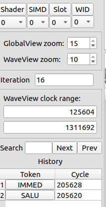
se_sm_sl_wv coordinate.真实的左侧控制面板:目标 Shader / SIMD / Slot / WID、 WaveView 时钟区间、 缩放、 loop 迭代导航、 搜索、 选择历史 —— 这些旋钮精确地选出一个 se_sm_sl_wv 坐标。 ROCm/rocprof-compute-viewer · docs/data/left.png06Timeline views · three ways to slice waves时间线视图 · 三种切 wave 的方式
The same trace, drawn three ways — by hardware slot, by instruction class, or all at once.同一份 trace,画三遍 —— 按硬件 slot、 按指令类别,或者全都画上。
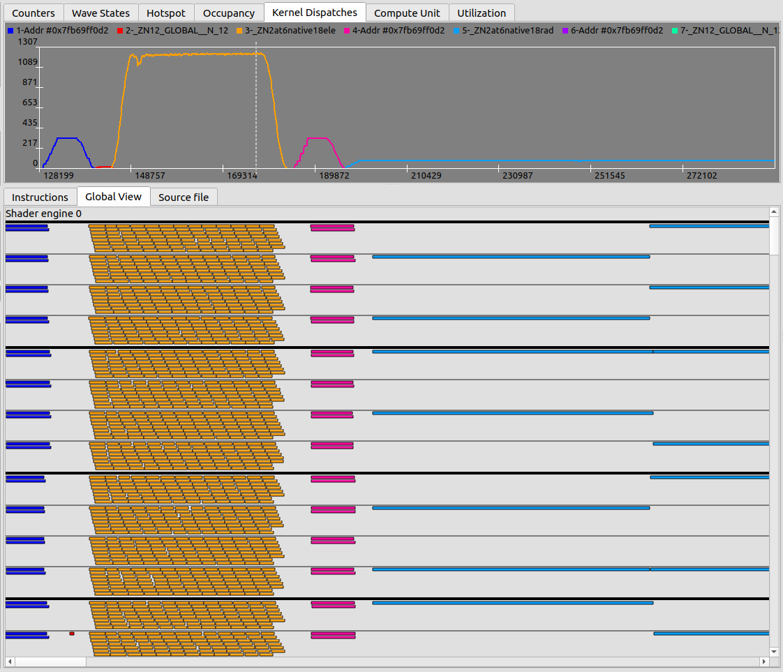
Global ViewGlobal View
The widest lens: every wave across all enabled Shader Engines, each color-coded by kernel. Use it to see how waves pack in time — long tails, stragglers, a kernel that never overlaps with its neighbor.最广的镜头:所有启用的 Shader Engine 上的每个 wave,按 kernel 着色。 用它看 wave 在时间上怎么排布 —— 长尾、 掉队者、 某个永远不和邻居重叠的 kernel。
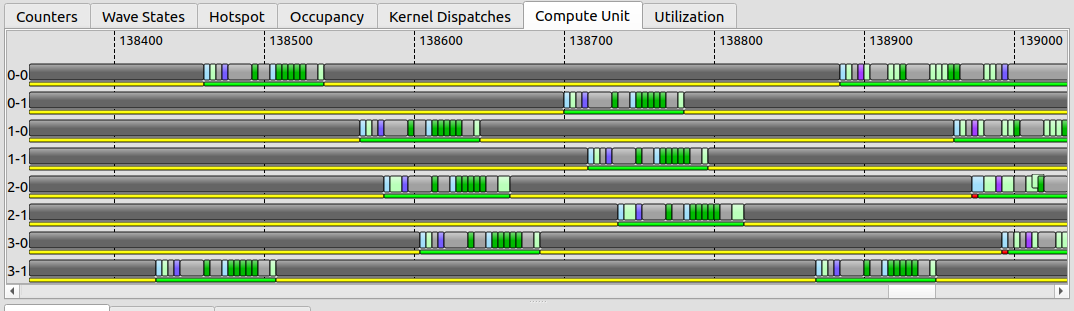
Compute Unit ViewCompute Unit View
The trace separated per SIMD-slot (the docs note ranges like 2–6), tracking individual wave execution. This is where you watch a single wave's life: when it was scheduled, when it ran, when it parked. A vertical slice of this tab is the Wave States plot.把 trace 按 SIMD-slot 拆开(文档里提到 2–6 这样的范围),追踪单个 wave 的执行。 这里你看一个 wave 的一生:何时被调度、 何时在跑、 何时停泊。 这个 tab 的一条竖切片,就是 Wave States 曲线。
Utilization ViewUtilization View
The trace drawn per instruction class — VALU, VMEM, SCALAR, OTHER — with immediate instructions and stall gaps hidden. This is the fastest read on what kind of work dominates: a wall of cyan (VMEM) says memory-bound; a wall of green (VALU) says compute-bound; mostly gaps says you are stalled and the ISA view will tell you on what.把 trace 按指令类别画 —— VALU、 VMEM、 SCALAR、 OTHER —— 隐藏掉立即数指令和 stall 空隙。 这是判断「什么活占主导」最快的一眼:一墙 cyan(VMEM)说明 memory-bound;一墙绿(VALU)说明 compute-bound;大片空隙说明你在 stall,而 ISA 视图会告诉你卡在什么上。
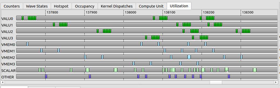
When the lanes go quiet (shaded), no instruction issued — the wave is waiting. The Utilization view shows the shape of the stall; the ISA view names its cause.当泳道安静下来(阴影处),没有指令发射 —— wave 在等。 Utilization 视图给你 stall 的 形状;ISA 视图给你它的 成因。
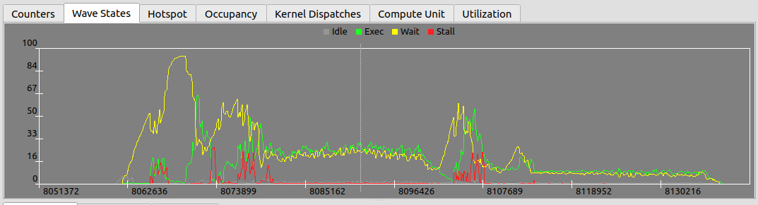
Not a mock-up — this is one real wave from an ATT capture on this MI350X. Two of the decoder's wave-states hold 97% of its 8480-cycle life; the viewer color-codes these in its Wave-States legend, and the Compute Unit view draws all 483 segments in order. This is the raw material every panel above is built from.不是示意图 —— 这是这台 MI350X 上一次 ATT 采集里真实的一个 wave。 decoder 的两个 wave-state 占了它 8480 个 cycle 生命的 97%;viewer 在 Wave-States 图例里给它们着色, Compute Unit 视图把全部 483 个 segment 按序画出。 这就是上面每块面板的原料。
07ISA view · where cycles are spentISA 视图 · cycle 花在哪
The instruction listing is the heart of RCV. Two numbers per line — Hitcount and Latency — and a set of arrows that explain the waits.指令列表是 RCV 的心脏。 每行两个数 —— Hitcount 和 Latency —— 再加一组解释「等待」的箭头。
The Instructions View lists the kernel's machine instructions with, per line:Instructions View 列出 kernel 的机器指令,每行带:
| Column | Meaning · how to read it |
|---|---|
| 列 | 含义 · 怎么看 |
Hitcount | how many times the instruction was issued — loop bodies and hot paths light up这条指令被发射了多少次 —— loop 体和热点路径会亮起来 |
Latency | accumulated cycles attributed to the line — a high-latency, low-hitcount line is a single expensive wait归到这一行的累计 cycle —— 高 latency、 低 hitcount 的行,是一次昂贵的等待 |
| source源码 | the correlated source line, when debug symbols are present关联的源码行(有 debug 符号时) |
The detail that separates RCV from a flat disassembly: memory-to-waitcnt dependency arrows, drawn per-wave, linking a memory operation to the s_waitcnt that later blocks on it. On AMD the cost of a load is rarely on the load — it is on the s_waitcnt vmcnt/lgkmcnt that stalls until the data lands. The arrow makes that causal pair visible: a fat latency bar on a s_waitcnt with an arrow reaching back to a global_load is the textbook memory-latency stall.把 RCV 和一份扁平反汇编区分开的细节:memory 到 waitcnt 的依赖箭头,按 wave 画出,把一次 memory 操作连到后面 block 在它上面的那条 s_waitcnt。 在 AMD 上,一次 load 的开销很少落在 load 本身 —— 它落在那条 stall 到数据返回为止的 s_waitcnt vmcnt/lgkmcnt 上。 这个箭头把这对因果关系画了出来:一条 s_waitcnt 上挂着粗 latency bar,又有箭头指回某条 global_load —— 这就是教科书式的 memory-latency stall。
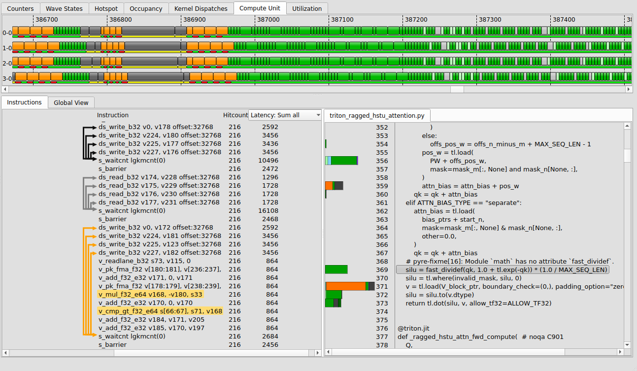
s_waitcnt dependency arrows on the left gutter. The fat-latency line with an arrow back to its load is the stall you are hunting.真实的 ISA 视图:每条指令一列 Hitcount 与 Latency、 反汇编、 关联的源码, 以及左侧栏里 per-wave 的 memory 到 s_waitcnt 依赖箭头。 那条粗 latency、 又有箭头指回它 load 的行,就是你在找的 stall。 ROCm/rocprof-compute-viewer · docs/data/isaview.pngHotspot TabHotspot Tab
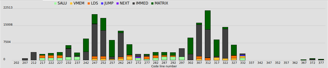
A histogram of total accumulated latency cycles per bin, based on the bin's center value, computed across all waves in the selected clock range. Where the ISA view is per-line, the Hotspot tab is the distribution — it tells you whether the cost is one fat outlier or smeared across many lines.一张直方图:每个 bin 的累计 latency cycle 总量(按 bin 中心值统计),在所选时钟区间内对所有 wave 计算。 ISA 视图是逐行的,Hotspot tab 则是分布 —— 它告诉你开销是一个肥尾的离群点,还是摊在很多行上。
A real case — 43% LDS-wait in a kernel with no LDS一个真实案例 —— 一个没有 LDS 的 kernel,却有 43% 的 LDS-wait
Back to the same topk_gating_softmax kernel from Plate VI. Its ATT trace stalls 132.3K of 272.7K cycles (48.5%), and 43.4% of that is s_waitcnt lgkmcnt(0) — the LDS/SMEM-wait bucket. Except the kernel has no LDS: ds_read: 0, ds_write: 0. So what waits on the LGKMCNT fence? The cross-lane shuffle_xor butterflies — on CDNA they lower to ds_swizzle_b32 / ds_bpermute_b32, which retire on LGKMCNT exactly like an LDS op. topk=6 means six serial argmax reductions plus a max and a sum, each a 3-step butterfly ending on an LGKMCNT drain — so nearly half the runtime is threads waiting on the lane-shuffle network, not memory. You would never see this in the source or an instruction count; only the ATT wave-state plus per-instruction view exposes it. (And the per-line table is useless here: 98% collapses onto the @flyc.kernel line — the §11 problem, in the wild.)回到 Plate VI 里那个 topk_gating_softmax kernel。 它的 ATT trace 在 272.7K cycle 里 stall 了 132.3K(48.5%), 其中 43.4% 是 s_waitcnt lgkmcnt(0) —— LDS/SMEM-wait 桶。 可这个 kernel 没有 LDS:ds_read: 0, ds_write: 0。 那在 LGKMCNT fence 上等的是什么? 是跨 lane 的 shuffle_xor 蝶形归约 —— 在 CDNA 上它们下沉成 ds_swizzle_b32 / ds_bpermute_b32, 和真正的 LDS 访问一样在 LGKMCNT 上退休。 topk=6 意味着六趟串行 argmax 归约, 外加一次 max 和一次 sum, 每趟是 3 步蝶形、 每步以一次 LGKMCNT drain 收尾 —— 于是近一半的运行时间是线程在等 lane-shuffle 网络, 不是在等访存。 你在源码里看不到、 在指令计数里也看不到;只有 ATT 的 wave-state 加 per-instruction 视图才能挖出来。 (而这里的逐行表是没用的:98% 塌缩到 @flyc.kernel 那一行 —— §11 那个问题的真身。)
08Counters, plots & summary计数器、 曲线与汇总
The trace is one wave deep; the counter and occupancy plots give you the breadth around it.trace 只有一个 wave 的深度;计数器和 occupancy 曲线给你它周围的广度。
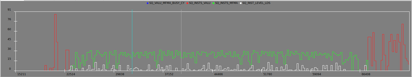
Counters TabCounters Tab
Plots hardware performance counters — up to 8 SQ counters — alongside the trace, with support for user-defined derived counters you can edit in place. This is how cache-hit or issue-rate context lands on the same x-axis as the instruction stream.把硬件性能计数器 —— 最多 8 个 SQ 计数器 —— 和 trace 画在一起,并支持你就地编辑的 自定义派生计数器。 cache 命中率或发射率这类上下文,就是这样落到和指令流同一条 x 轴上的。
Wave States · Occupancy · DispatchesWave States · Occupancy · Dispatches
- Wave States — a vertical slice of the Compute Unit tab: what state each wave is in at a given instant.Wave States —— Compute Unit tab 的一条竖切片:某一时刻每个 wave 处于什么状态。
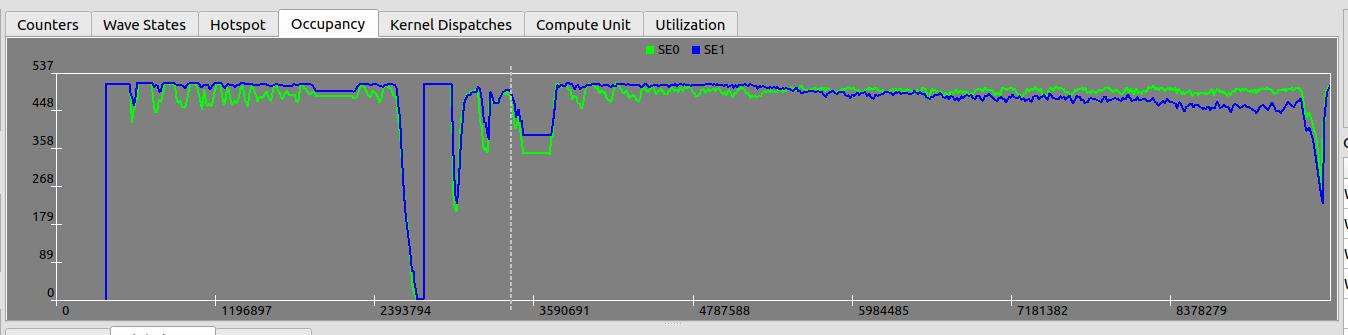
- Occupancy — occupancy per Shader Engine, in number of waves. The classic "are we filling the machine" plot.Occupancy —— 每个 Shader Engine 的 occupancy,以 wave 数计。 经典的「机器填满了吗」曲线。
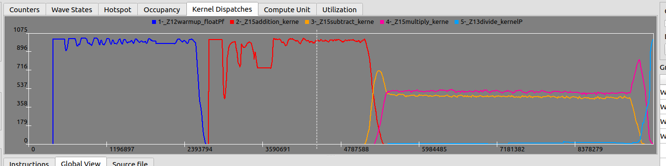
- Dispatches — occupancy per kernel, so you can attribute the fill to a specific launch.Dispatches —— 每个 kernel 的 occupancy,这样你能把「填充」归到某次具体的 launch。
Summary ViewSummary View
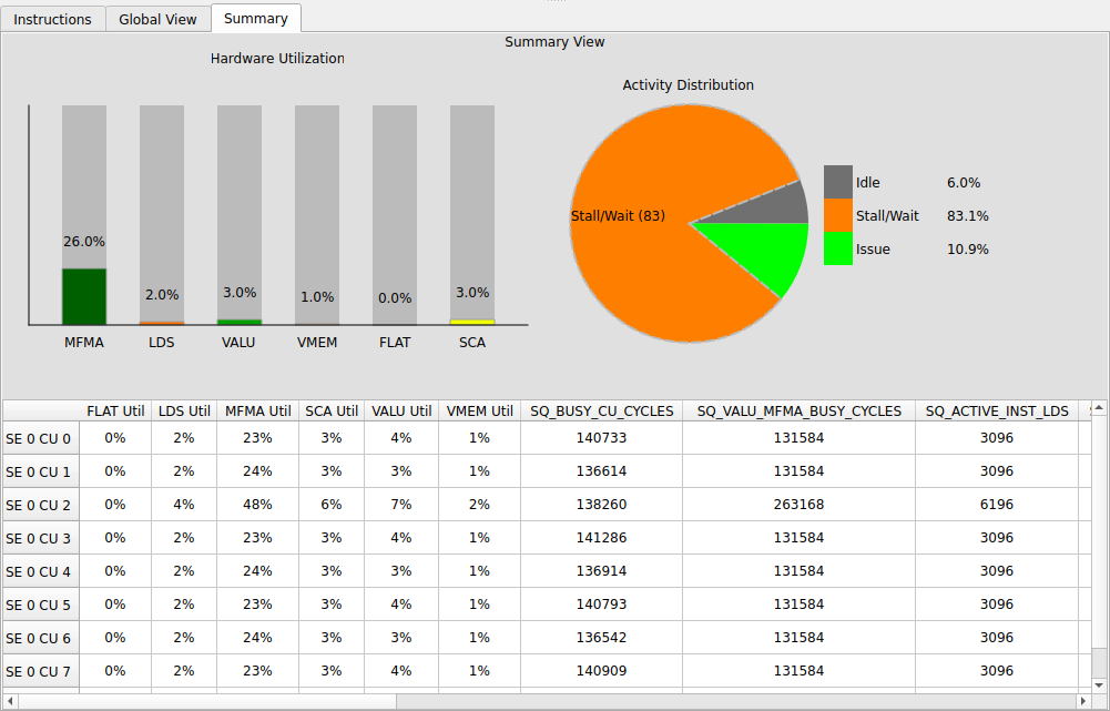
On MI2xx / MI3xx parts, a rolled-up panel: average instruction cost, hardware utilization by type, per-compute utilization. It is the bridge back to the aggregate world — the number you would quote in a report, derived from the same trace you just walked instruction by instruction.在 MI2xx / MI3xx 上,一个汇总面板:平均指令开销、 按类型的硬件利用率、 per-compute 利用率。 它是回到聚合世界的桥 —— 你写进报告里的那个数,正是从你刚刚逐条走过的那份 trace 里算出来的。
09A reading loop一套阅读流程
"This kernel is slow" → a source line, in five clicks.「这个 kernel 慢」→ 一行源码,五次点击搞定。
- Explorer — sort by the latency bar; open the file with the longest one.Explorer —— 按 latency bar 排序;打开最长的那个文件。
- Utilization — is the dominant color VMEM (memory-bound), VALU (compute-bound), or mostly gaps (stalled)?Utilization —— 主色是 VMEM(memory-bound)、 VALU(compute-bound),还是大片空隙(stall)?
- Compute Unit — pick one representative wave; scope its clock range in the side panel.Compute Unit —— 挑一个有代表性的 wave;在 side panel 里圈定它的时钟区间。
- ISA — sort by Latency; the fat line is the cost. Follow its waitcnt arrow to the load it waits on.ISA —— 按 Latency 排;肥行就是开销。 顺着它的 waitcnt 箭头找到它在等的那次 load。
- Source — click the line; fix the access pattern, the tiling, or the dependency. Re-capture and diff the latency.Source —— 点开那行;改访存模式、 tiling 或依赖。 重新采集,diff latency。
s_waitcnt lgkmcnt(0) with the arrow reaching a ds_read/ds_write is the LDS-latency signature — the same one the project's lds-optimization skill chases with swizzle/padding.一条肥 s_waitcnt lgkmcnt(0),箭头指向 ds_read/ds_write,就是 LDS-latency 的签名 —— 也正是项目里 lds-optimization skill 用 swizzle / padding 去追的那个。Read it without the GUI不开 GUI 也能读
The viewer is where you look; it is not where you triage. A 200-line script — hotspot_analyzer.py in flydsl-kernel-profiling/tools — reads the same code.json the viewer reads and prints the kernel's whole story with no clicks: it classifies each instruction's stall by mnemonic (vmcnt → VMEM-wait, lgkmcnt → LDS/SMEM-wait, ds_read → LDS, v_mfma → MFMA), aggregates by source line, and ranks the top-K by stall cycles with a dominant-type column. One table answers the only question that matters first — memory, sync, or compute? — and tells you whether opening the GUI is even worth it.viewer 是用来 看 的, 不是用来 分诊 的。 一个两百行的脚本 —— flydsl-kernel-profiling/tools 里的 hotspot_analyzer.py —— 读的是和 viewer 完全相同的 code.json, 不点一下鼠标就打印出整个 kernel 的故事:它按助记符给每条指令的 stall 分类(vmcnt → VMEM-wait、 lgkmcnt → LDS/SMEM-wait、 ds_read → LDS、 v_mfma → MFMA), 按源码行聚合, 再用 stall cycle 排出 top-K 并附上 dominant-type 一列。 一张表先回答最该先问的:卡在访存、 同步, 还是计算? 也顺带告诉你这个 GUI 到底值不值得打开。
run_pool.py is the whole scheduler in ~70 lines (a free-GPU list, a kernel queue, Popen + poll + reap, no locks). A 17-kernel sweep that is 50+ minutes serial collapses to ~3 batches on 8 GPUs. The single-CU limit that makes ATT awkward to read is exactly what makes it embarrassingly parallel to capture.ATT 每次 dispatch 只追一个 CU, 还要独占 GPU —— 听着像串行化的代价, 其实正相反。 一卡一 kernel, 退出就把卡还回空闲池:run_pool.py 整个调度器约 70 行(一个空闲 GPU 列表、 一个 kernel 队列、 Popen + poll + reap, 无锁)。 串行要 50 多分钟的 17-kernel 扫描, 在 8 卡上压成约 3 个批次。 让 ATT 难 读 的单 CU 限制, 恰恰让它的 采集 尴尬地并行。10The source · how RCV is built源码 · RCV 怎么搭起来的
A Qt desktop app with a pluggable decode-and-disassemble back end.一个 Qt 桌面程序,后端是可插拔的「解码 + 反汇编」。
RCV (ROCm/rocprof-compute-viewer, branch amd-mainline) is built with CMake on Qt 5 or 6 (default Qt 6.8), and ships for Linux, macOS, and Windows. The decode/disassembly back end is what changes with build flags:RCV(ROCm/rocprof-compute-viewer,分支 amd-mainline)用 CMake 构建,基于 Qt 5 或 6(默认 Qt 6.8),发布到 Linux、 macOS、 Windows。 随构建开关变化的,是解码 / 反汇编后端:
- JSON-only build — just Qt base + standard tooling; opens decoded
ui_outputdirectories. The lightest path.仅 JSON 构建 —— 只要 Qt base + 标准工具链;打开已解码的ui_output目录。 最轻量的路径。 - ATT / ROCPD support — links
rocprof-trace-decoder(V2 API, SOVERSION 0.2) to decode raw.attin-app, plus LLVM-C as the default disassembly backend (amd_comgris the legacy alternative).ATT / ROCPD 支持 —— 链接rocprof-trace-decoder(V2 API,SOVERSION 0.2)在程序内解码原始.att,外加 LLVM-C 作默认反汇编后端(amd_comgr是旧的备选)。
So the dependency you most often hit is the decoder: a JSON-only viewer reads what rocprofv3 already decoded, while the full build can chew raw SQTT itself. rocprofv3 in turn is part of rocprofiler-sdk — and both repos are open, which is the whole reason this reading can be precise rather than hand-wavy.所以你最常撞上的依赖就是这个 decoder:仅 JSON 的 viewer 读 rocprofv3 已经解码好的东西,而完整构建能自己啃原始 SQTT。rocprofv3 这边则属于 rocprofiler-sdk —— 两个仓库都开源,这正是这篇阅读能精确、 而不是空谈的全部原因。
11IR → Python · whose line is it?IR → Python · 这是谁的行?
The ISA view's source column is only as good as the Location every IR op carries. FlyDSL learned this the hard way — and so did I, with a PR that got closed.ISA 视图的源码列, 好不好全看每个 IR op 带着的那个 Location。 FlyDSL 是吃了苦头才懂的 —— 我也是, 一个被关掉的 PR。
Everything in §07 assumes one thing: that each machine instruction can be traced back to a source line. That only works if every MLIR op in the kernel carries a debug Location (hence FLYDSL_DEBUG_ENABLE_DEBUG_INFO=1 at capture). The viewer is a passive reader here — it shows whatever Location the IR baked in. So if the mapping is useless, the fix is not in the viewer; it is upstream, in how the compiler stamps locations.§07 里的一切都假设了一件事:每条机器指令都能回溯到一行源码。 这只有在 kernel 里每个 MLIR op 都带着 debug Location 时才成立(所以采集时要 FLYDSL_DEBUG_ENABLE_DEBUG_INFO=1)。 viewer 在这里是被动读者 —— IR 里烤进了什么 Location, 它就显示什么。 所以如果映射没用, 修的地方不在 viewer, 而在上游 —— 在编译器怎么盖 location 戳。
FlyDSL is a Python → MLIR → ISA compiler, and it broke exactly here. For flash_attn_func debug info was present and 2069/2070 ISA rows mapped to Python — but 91.9% of instructions collapsed onto flash_attn_func.py:257, the @flyc.kernel decorator line, and 6.3% onto :283, a one-line _mfma helper. The trace mapped, but to a line you cannot act on. Root cause: the schedule emits its DMA / MFMA / wait / barrier ops from nested helper closures, so the tracer's _caller_location(depth=1) lands on the helper body, and untraced sync ops fall through to the kernel-default line.FlyDSL 是一个 Python → MLIR → ISA 的编译器, 它恰恰就在这里坏了。 对 flash_attn_func, debug info 是有的, 2069/2070 行 ISA 都映射到了 Python —— 但 91.9% 的指令塌缩到了 flash_attn_func.py:257, 也就是 @flyc.kernel 装饰器那一行, 另有 6.3% 落到 :283, 一个一行的 _mfma helper。 trace 映射上了, 但映射到了一行你没法据此动手的代码。 根因:schedule 的 DMA / MFMA / wait / barrier 是从嵌套 helper 闭包里发出来的, 于是 tracer 的 _caller_location(depth=1) 落在 helper 体上, 而未被 trace 的同步 op 则掉到 kernel 的默认行。
Real numbers from the PR. Before: latency piled on the @flyc.kernel line; 6 distinct source lines. After the right fix: spread across the helper statements; 29 distinct lines. Same trace, same viewer — only the Locations in the IR changed.来自 PR 的真实数字。 修复前:latency 全堆在 @flyc.kernel 那一行;只有 6 个不同源码行。 用对的修法之后:摊到各 helper 语句上;29 个不同行。 同一份 trace、 同一个 viewer —— 变的只是 IR 里的 Location。
The wrong fix — my PR #593错的修法 —— 我的 PR #593
My first instinct (PR #593, fixes #587) was a source_loc context manager: pin the user call-site Location in a thread-local, and have the tracer consult it first — loc = kwargs.pop("loc", None) or _pinned_loc() or _caller_location(depth=1). It worked, partially: distinct lines went 6 → 29. But ~54% still sat on the function line, and worse, it was a manual annotation you had to wrap around every schedule helper, kernel by kernel.我的第一反应(PR #593, 修 #587)是一个 source_loc context manager:把用户 call-site 的 Location 钉在 thread-local 里, 让 tracer 先查它 —— loc = kwargs.pop("loc", None) or _pinned_loc() or _caller_location(depth=1)。 它部分有效:不同行数从 6 涨到 29。 但仍有约 54% 留在函数那一行, 更糟的是, 它是一个你得 kernel 一个个、 把每个 schedule helper 包起来的手动标注。
The right fix — #586's WrapLocations对的修法 —— #586 的 WrapLocations
PR #586 (merged) added a WrapLocations pass in compiler/ast_rewriter.py that wraps every statement inside the nested schedule helpers. Each DMA / MFMA / wait / barrier op then gets its own helper line automatically — for all kernels, with no annotation. It is a compiler-side transform, not a user contract. That is the difference: location attribution is a property the IR pipeline should produce, not something the kernel author should have to declare.PR #586(已合并)在 compiler/ast_rewriter.py 里加了一个 WrapLocations pass, 把嵌套 schedule helper 里面的每一条语句都包起来。 于是每个 DMA / MFMA / wait / barrier op 自动拿到自己的 helper 行 —— 对所有 kernel、 零标注。 它是编译器侧的变换, 不是一份用户契约。 这就是分水岭:location 归属应该是 IR 管线产出的属性, 而不是 kernel 作者要去声明的东西。
source_loc re-pin actively fought #586 (mixed attribution — untraced ops to the helper line, traced ops to the call site). I closed #593 in favor of #586. The better PR was the one that pushed the fix down into the pass pipeline instead of up into the API.maintainer(@coderfeli)点了一句:「#586 会帮上吗?」 帮上了 —— 而且它让 #593 不只是多余, 还有害:#586 已经把每条语句都包了, 所以那些同步 wrapper 是重复的, 而 source_loc 的重新钉位还在主动跟 #586 打架(归属错乱 —— 未 trace 的 op 去 helper 行, trace 的 op 去 call site)。 我把 #593 关掉, 让位给 #586。 更好的那个 PR, 是把修复压到 pass 管线里、 而不是抬到 API 上的那个。The takeaway loops back to the viewer: RCV's source column is downstream of all this. When your FlyDSL ATT trace finally points at the right line, thank a compiler pass — not the profiler.这个教训绕回到 viewer:RCV 的源码列是这一切的下游。 当你的 FlyDSL ATT trace 终于指对了行, 该谢的是一个编译器 pass —— 不是 profiler。
12Reefs暗礁
Where ATT readings go quietly wrong.ATT 会悄悄读错的地方。
att_buffer_size drops the tail of the trace with no error. If a wave's timeline ends abruptly, raise the buffer (0x6000000 → 0xC000000) before trusting the picture.att_buffer_size 太小会把 trace 尾部丢掉,且不报错。 如果某个 wave 的时间线戛然而止,先把 buffer 加大(0x6000000 → 0xC000000)再相信这张图。att_target_cu = 1 you trace one CU's waves. If work is unbalanced across CUs, that slice may not be representative — widen simd_select/shader_engine_mask deliberately when in doubt.设了 att_target_cu = 1,你追踪的是一个 CU 的 wave。 如果各 CU 之间负载不均,这个切片可能不具代表性 —— 拿不准时,有意识地放宽 simd_select/shader_engine_mask。host_trap/time only. It estimates where the PC sits; it does not give you the waitcnt arrows. Reach for ATT when you need causality, PC sampling when you need cheap coverage.PC sampling 是统计性的,目前只有 host_trap/time。 它估计 PC 停在哪;给不了 waitcnt 箭头。 需要因果关系时用 ATT,需要便宜的覆盖面时用 PC sampling。dispatch_<N> suffix is the process-wide HSA dispatch counter, not your kernel's index. It counts every launch in the process — including torch utility kernels (vectorized_elementwise_kernel, reduce_kernel) that never match your regex. Run your kernel 12× and you may get dispatch_234, 236, 238… with the odd slots taken by torch. The gaps are normal; nothing was dropped.dispatch_<N> 后缀是进程级的 HSA dispatch 计数器, 不是你 kernel 的序号。 进程里每次 launch 它都加一 —— 包括那些永不匹配你 regex 的 torch 工具 kernel(vectorized_elementwise_kernel、 reduce_kernel)。 你的 kernel 跑 12 次, 可能拿到 dispatch_234, 236, 238…, 奇数槽被 torch 占走。 跳号是正常的, 什么都没丢。kernel_iteration_range "[N, [M-M]]" looks like "capture exactly iteration M." In rocprofv3 v1.1 the inner bound is a lower bound: if the ATT buffer still has slack, it also grabs the next matching dispatch. So [8-8] reliably yields two full, valid traces of the same kernel at the same steady-state iteration. Reads like a duplicate bug; it is a free noise-floor check — if the two stall breakdowns agree within a few percent, your steady state is stable.kernel_iteration_range "[N, [M-M]]" 看着像「只采迭代 M」。 在 rocprofv3 v1.1 里, 内层界限是下界:只要 ATT buffer 还有余量, 它会把下一个匹配的 dispatch 也抓进来。 于是 [8-8] 稳定给出同一 kernel、 同一稳态迭代的两份完整有效 trace。 看着像重复 bug, 其实是白送的噪声底检查 —— 两份 stall 分布若相差几个百分点以内, 说明稳态是稳的。ui_output_agent_*_dispatch_<N> placeholders before collection starts: they carry code.json / filenames.json with zero waves and an empty instruction array, and appear when the grid is too small to ever occupy the single target CU. They look like real captures but contain nothing. Detect with waves == 0 (no se*_sm*_*.json files) and delete — keep the dispatch ranked highest on (waves, instructions, mapped).rocprofv3 在采集开始前会预分配 ui_output_agent_*_dispatch_<N> 占位符:它们带着 code.json / filenames.json, 但 wave 数为零、 指令数组为空, 在 grid 太小、 根本占不满那唯一目标 CU 时出现。 看着像真采集, 实则啥都没有。 用 waves == 0(没有 se*_sm*_*.json 文件)检出并删掉 —— 只留在 (waves, instructions, mapped) 上排名最高的那个。13Epilogue尾声
The reason ATT is worth the ceremony — the narrow window, the separate runs, the buffer math — is that it closes the loop between a number and a line of code. A roofline tells you a kernel is memory-bound; the ISA view shows you the exact s_waitcnt that ate the cycles and the global_load it waited on. One is a verdict, the other is an address. Optimization happens at the address.ATT 值得这套仪式 —— 窄窗口、 分开运行、 buffer 的算术 —— 的理由,是它把一个数字和一行代码之间的环闭上了。 roofline 告诉你某个 kernel 是 memory-bound;ISA 视图给你那条吃掉 cycle 的 s_waitcnt,以及它在等的那次 global_load。 前者是判决,后者是地址。 优化发生在地址上。
On this MI350X, every FlyDSL kernel in flydsl-kernel-profiling already carries an att_viewer/ directory of exactly these traces. The tools are open; the traces are on disk; the only missing step is learning to read the panel — which, now, you can.在这台 MI350X 上,flydsl-kernel-profiling 里每个 FlyDSL kernel 都已经带了一个装着这种 trace 的 att_viewer/ 目录。 工具是开源的,trace 在磁盘上,唯一缺的一步是学会读这个面板 —— 而现在,你会了。